
mojo's Blog
Cross-Validation 본문
Cross-Validation
※ Hold-out Method
Divide a given data into a training set and a test set.
- The training set and the test set should NOT overlap each other.
How to choose a good model?
- With the training set, build each model.
- With the test set, evaluate each model.
- Choose the model which shows the best performance with the test set.
훈련용 데이터와 테스트용 데이터는 중복이 허용되면 안된다.
훈련용 데이터를 통해 학습이 완료된 모델을 통해 테스트용 데이터를 평가하여 얼마나 정확한지
평가를 하며, 각각의 모델을 통해 어떤 모델이 최고의 성능을 내는지 찾는것이 목적이다.
Size of the test set : Usually 30 ~ 50 % of given datasets
30 ~ 50 이라는 수치가 꼭 정답은 아니지만, 적당한 데이터를 활용하여 테스트용으로 쓰면 된다.
Advantage
- Simple and easy
Disadvantage
- Waste of data : The test set is not used for building a model
- Random split : Evaluation can be significantly different depending on data split
랜덤하게 훈련용 데이터와 테스트용 데이터를 분리하는데,
훈련용 데이터 셋에 지나치게 데이터가 몰리는 경향이 존재할 수 있으며 자연스럽게
테스트용 데이터 셋에 다른 성격의 데이들로 구성될 수 있다.
※ Cross Validation
Cross-validation (\(k\) - fold)
- Data D is randomly partitioned into \(k\) mutually exclusive subsets {\(D_{1}, ..., D_{k}\)},
with approximately equal size.
Overall procedure
- The data is partitioned into \(k\) groups.
\(k - 1\) of the groups are used for training the model.
One remaining group is used for evaluating the model.
- Repeat procedure for all \(k\) choices.
- Performance from the \(k\) runs are averaged.

위와 같이 \(k\) 개의 그룹으로 분할하여 \(k - 1\) 개의 그룹은 훈련용 데이터로 분류하고,
나머지 \(1\) 개의 그룹은 테스트용 데이터로 분류한다.
그리고 총 \(k\) 번 만큼 모델들을 학습시키면서 가장 성능이 좋게 나온 모델을 선정하는 방식이다.
Summary
The data set is divided into \(k\) subsets, and the hold-out method is repeated \(k\) times
Each time, one of the \(k\) subsets is used as the test set and the other \(k - 1\) subsets
are put together to form a training set.
The average error across all \(k\) trials is computed.
The variance is reduced as \(k\) is increased..
Advantage
- Less dependent on how the data gets divided.
- Every data point gets to be in a test set exactly once and gets to be in a training set \(k - 1\) times.
Disadvantage
- Time
\(k\) 개의 그룹으로 나눠서 data 를 공정하게 참여시킴으로써 좀 더 엄밀한 평가를 할 수 있는 장점이 있다.
하지만 그룹을 분할한 횟수 만큼 iteration 을 돌면서 훈련시키기 때문에 시간이 많이 든다는 단점이 있다.
※ Leave-one-out Cross Validation (LOOCV)
Extreme case of k-fold cross validation
- If data size is \(n\), set \(k = n\).
- Every data point except one is used for training and the remaining one is used for testing.
- Repeat this \(n\) times.
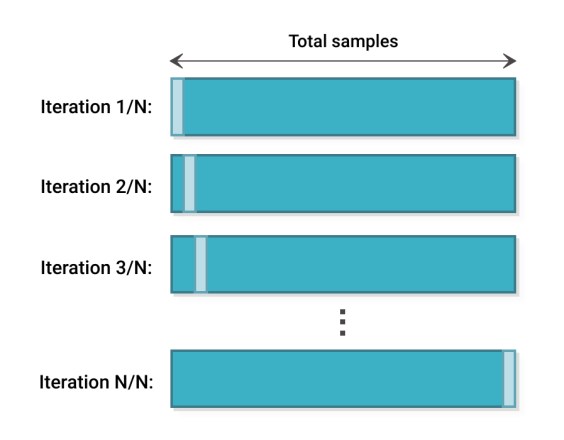
위 경우는 \(n - 1\) 개의 데이터가 훈련용 데이터, \(1\) 개의 데이터가 테스트용 데이터로 분리된다.
그리고 \(n\) 번만큼 iteration 을 돌면서 모델을 학습시킨다.
이러한 극단적인 케이스는 데이터가 충분하지 않은 경우에 대해서 위와 같은 방식을 사용할 수 있다.
그러나 데이터가 충분히 많은 경우, \(k\) 를 5 또는 10 으로 할 수 있고 일반적으로 10 을 한다.
※ Three Datasets for Evaluation
Training dataset
- The sample of data used to fit the model
Validation dataset
- The sample of data used to provide an unbiased evaluation of a model fit on the training dataset
while tuning model hyperparameters
Test dataset
- The sample of data used to provide an unbiased evaluation of a final model fit on the training dataset
실제로 모델을 학습하는 과정에서 overfitting 되었는지 안되었는지 확인이 필요하다.
따라서 위와 같이 데이터셋을 3가지로 분류하여 평가가 이뤄지게 된다.
예를 들어서 데이터가 100개 있을 경우, training 데이터셋 72 개, validation 데이터셋 8 개,
test 데이터셋 20 개로 같이 분리할 수 있다.
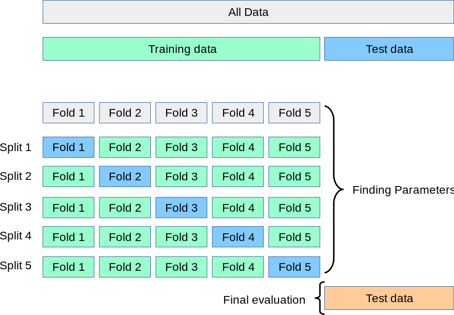
위 사진과 같이 training 데이터와 test 데이터를 분리시키고,
training 데이터 안에서 validation 데이터를 \(k = 5\) 개 만큼 또 분리하여 모델을 학습시키고
그 중에서 가장 좋은 모델을 선정하여 선정된 모델을 통해 test 데이터를 predict 하게 된다.
Evaluation Metrics
※ Evaluation Metrics in Regression Models
Mean absolute error (MAE) and mean squared error (MSE)
\(MAE = \frac{1}{n}\sum_{i=1}^{n}|f(x^{(i)}) - y^{(i)}| \)
\(MSE = \frac{1}{n}\sum_{i=1}^{n}(|f(x^{(i)}) - y^{(i)}|)^{2}\)
Root mean squared error (RMSE)
- MSE is more popular than MAE because MSE punishes larger errors.
- RMSE is even more popular than MSE because RMSE is interpretable in the "y" axis.
\(RMSE = \sqrt{MSE} = \sqrt{\frac{1}{n}\sum_{i=1}^{n}(|f(x^{(i)}) - y^{(i)}|)^{2}}\)
※ Confusion Matrix
Building a confusion matrix for actual and predicted results
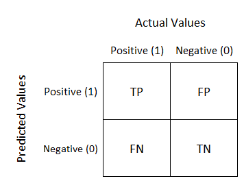
This can be used to measure accuracy, precision, recall, and so on.
위 경우는 binary classification 에 대한 confusion matrix 이다.
confusion matrix 을 활용하여 다양한 값들을 평가할 수 있다.
TP, TN 는 모델이 맞게 예측한 것이고 FP, FN 는 모델이 틀리게 예측한 것이다.
FP 는 positive 을 예측했지만 negative 이 정답인 경우고,
FN 는 negative 을 예측했지만 positive 이 정답인 경우이다.
※ Accuracy, Error Rates
The fraction of correct classification results
\(accuracy = \frac{TP + TN}{TP + FP + FN + TN}\)
\(error_rate = 1 - accurcay\)
\(TP + FP + FN + TN\) 는 주어진 테스트 데이터 전부를 의미하고,
\(TP + TN\) 는 실제로 테스트 데이터 중 모델이 맞춘 개수를 의미한다.
그러나 accuracy가 높다고 항상 좋은 모델이라고 단정지을 수는 없다.
그러한 케이스를 살펴보도록 하자.
※ Example: Why not just Use Accuracy?
99.9% of documents are irrelevant in most of the cases
- Labeling every document as irrelevant has high accuracy but it is useless in the Web search engine
People want to find something that are tolerant for junk.
임의의 질의에 대해서 전체 문서 중에 관련 있는 문서는 매우 극소수이다. (0.1%)
이러한 케이스로 accuracy 를 평가할 때 모든 질의에 대해 전부 negative 라고 한다면
negative 부분은 다 맞추었기 때문에 99.9% accuracy 를 가질 수 있게 된다.
하지만 0.1 %가 일부 틀릴 수도 있지만, 보유하고 있는 문서들을 최대한 많이 보여주는 그런 검색 엔진이
좋은 검색 엔진이라고 볼 수 있다.
정리하자면 positive, negative 의 비율이 imbalance 한 그런 환경에서는 효과적이지 않다고 볼 수 있다.
위와 같은 케이스를 평가하기 위해 Precision, Recall 이 등장하게 된다.
※ Precision and Recall
Precision
- Exactness : How many selected items are relevant?
\(Precision = \frac{TP}{TP+FP}\)
Recall
- Completeness : How many relevant items are selected?
\(Recall = \frac{TP}{TP+FN}\)
The perfect score of both measures is 1.0
- In general, the inverse relationship between precision and recall.
precision, recall 은 서로 trade off 관계를 가지고 있다.
precision 성능이 좋을 경우 recall 의 성능이 떨어질 수 있게 되고 ,
recall 의 성능이 좋을 경우 precision 의 성능이 떨어질 수 있게 된다.
※ F-Measure (F-Score)
F-mesaure (F1 or F-score)
- The weighted harmonic mean of precision and recall
\(F = \frac{1}{\alpha \frac{1}{P} + (1 - \alpha)\frac{1}{R}} = \frac{(\beta ^{2} + 1)PR}{\beta ^{2}P + R}\)
where \(\beta ^{2} = \frac{1 - \alpha}{\alpha}\)
- When \(\alpha = 0.5\) (i.e., \(\beta = 1.0\) )
\(F = \frac{2PR}{P+R}\)
Why harmonic mean?
- The harmonic mean is always less then or equal to the arithmetic mean and the geometric mean.
- When \(P\) and \(R\) differ greatly, the harmonic mean is closer to their minimum than
to their arithmetic mean
F-measure 는 precision, recall 에 대한 measure 를 합친 것으로 볼 수 있다.
일반적으로는 precision 과 recall 의 산술평균을 통해 구할 수 있다.
하지만 위와 같이 다른 방법으로 조화 평균을 사용할 수 있다.
조화 평균을 사용하는 이유는 precision, recall 둘 다 적당히 잘 높이는 부분이 중요하다는 걸
반영하기 위해 쓰는 것으로 볼 수 있다.
'머신러닝' 카테고리의 다른 글
| The Overfitting Problem (0) | 2023.04.03 |
|---|---|
| Multinomial Logistic Regression (0) | 2023.03.29 |
| The Concept of Logistic Regression (0) | 2023.03.29 |
| Parameter Estimation (0) | 2023.03.21 |
| Classification Problem (0) | 2023.03.19 |


