
mojo's Blog
Parameter Estimation 본문
※ Estimation in Statistics
Use sample statistics to estimate population parameters.
-> E.g., Sample means are used to estimate population means.
A point estimate of a population parameter is a single value of a statistic.
An interval estimate is defined by two numbers, between which a population
parameter is said to lie.
- \(a < x < b\) is an interval estimate of the population mean \(\mu \).
일반적으로 interval estimate 보다 point estimate 방식으로 parameter를 주로 추정한다.
※ Example: Cilantro-Haters
Experiment: Ask \(n\) random people to taste cilantro.
Model: \(X_{i} ~ Bernoulli(p)\) is whether the \(i\)-th person says it taste like soap.
Data: \(x_{1}, ..., x_{n}\) are the results of the experiment.
Inference: Estimate \(p\) from the data.
주어진 샘플이 베르누이로 표현될 때, 두 개의 이산값을 가진 분포로 이루어진다.
목적은 \(p\)값을 추정하는 것으로 볼 수 있다. (그렇지 않은 경우 : \(1 - p\))
For a given value of \(p\) the probability of getting 65 'successes' is the binomial probability.
The likelihood \(P(data | p) = \begin{pmatrix} 100 \\ 65\\ \end{pmatrix} p^{65}(1-p)^{35}\)
주어진 100명 중에 65명의 사람이 임의로 고수 맛을 느낀다고 했을 때, 주어진 데이터에 대해서
\(p\) 값을 추정하는 것이 문제이다.
이러한 문제를 해결하기 위해 위와 같이 Likelihood 함수를 이용하고 이를 최대화하는 방향의
\(p\) 값을 찾는것이다.
※ Maximum Likelihood Estimation (MLE)
It is a way to estimate the value of a parameter of interest.
Finding the value of \(p\) that maximizes the likelihood.
There are different methods of finding the maximum
(1) Calculus : Solve \(\frac{d}{dp} P(data|p) = 0\) for \(p\).
=> We should also check that the critical point is a maximum.
(2) Sometimes, the derivative is never 0.
=> It is at an endpoint of the allowable range.
일단 (2) 는 고려하지 않고 (1) 방법으로 미분해서 0이 되는 지점을 통해 최대값을 찾는 방식에 대해
살펴보도록 한다.
The MLE is computed by calculus.
\(\frac{dP(data|p)}{dp} = \binom{100}{65}(65p^{64}(1-p)^{35} - 35p^{65}(1-p)^{34}) = 0\)
A sequence of algebraic steps gives:
\((65p^{64}(1-p)^{35} - 35p^{65}(1-p)^{34})\)
\(\hat{p} = \frac{65}{100}\)
주어진 likelihood 를 미분하여 p 값이 0이 되는 지점을 찾는 것은 극점을 찾는 문제로 생각할 수 있다.
즉, \(p = \frac{65}{100}\) 일 때 likelihood 가 최대화되는 것으로 볼 수 있다.
※ Log Likelihood
Because the log function turns multiplication into addition,
it is convenient to use the log of the likelihood function.
Log likelihood \(= ln(likelihood) = ln(P(data|p))\)
Example )
The likelihood is \(P(data|p) = \binom{100}{65}p^{65}(1-p)^{35}\)
The log likelihood is \(ln\binom{100}{65} + 65ln(p) + 35ln(1-p)\)
계산을 좀 더 편리하게 하고자 Likelihood에 로그를 씌우는 방식이다.
The MLE is computed by calculus.
\(\frac{dP(data|p)}{dp} = \frac{65}{p} - \frac{35}{1-p} = 0\)
A sequence of algebraic steps gives:
\(\frac{65}{p} - \frac{35}{1-p} = 0\)
\(\hat{p} = \frac{65}{100}\)
결국 결과를 보면, 100명의 사람중 65명의 사람이 고수를 먹을 때 비누 맛을 느낀다고 했다.
이때 likelihood를 최대화하는 p는 주어진 식에서 \(\frac{65}{100}\) 으로 표현된다.
※ Example: Coin Tossing
There is a box including three coins, which give heads with probability
\(p = 1/3, 1/2,\) and \(2/3\).
We choose a coin from the box and tossed it 100 times, resulting in 65 heads and 35 tails.
What is the likelihood of this data for each coin?
The likelihood function \(p(D | p)\) is computed by:
\(p(D|p=1/3)=\binom{100}{65}\left ( \frac{1}{3} \right )^{65}\left ( \frac{2}{3} \right )^{35}\)
\(p(D|p=1/2)=\binom{100}{65}\left ( \frac{1}{2} \right )^{65}\left ( \frac{1}{2} \right )^{35}\)
\(p(D|p=2/3)=\binom{100}{65}\left ( \frac{2}{3} \right )^{65}\left ( \frac{1}{3} \right )^{35}\)
The maximum likelihood is \(p = 2/3\).
위와 같이 binomial distribution에 따라 각각의 확률값을 표현할 수 있다.
\(p\) 값에 따라서 위와 같이 likelihood 값이 달라지는 것을 알 수 있고, 마지막 likelihood 가
나머지 두 개보다 더 큰 확률값을 가짐을 확인할 수 있다.
Maximum Likelihood Estimation
※ Maximum Likelihood Estimation (MLE)
Finding \(\Theta \) that maximizes \(P(X_{1}, ..., X_{n}; \Theta )\)
(of the joint pdf for continuous random variables)
We have \(P(X_{i}; \Theta )\) for random variable
\(P(X_{1}, ..., X_{n}; \Theta) = \prod_{i}^{}P(X_{i}; \Theta )\)
\(logP(X_{1}, ..., X_{n}; \Theta) = \sum_{i}^{}logP(X_{i}; \Theta )\)
각각의 n개의 데이터는 서로 독립이다. (따라서 모든 확률의 곱으로 표현됨 - joint probability)
즉, n개의 데이터가 identically independent distributed(iid) 가정 하에 parameter \(\Theta\) 를
추정하는 것이 목적이다.
We take a derivative and set it to zero.
\(\frac{\partial }{\partial \Theta }log\sum_{i}^{}P(X_{i}; \Theta ) = 0\)
주어진 likelihood 함수를 최대화하는 극점을 찾기 위해 위와 같이 미분을 통해 0 이 되는 \(\Theta\) 값을 찾는다.
※ Likelihood vs. Log Likelihood
Log-likelihood is a monotonic(단조로운) function of the likelihood.
The maximum is achieved at the same point, albeit, in most cases with a lot less compuation.
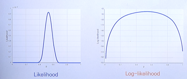
로그를 씌운다고 가장 최대화가 되는 지점은 변하지 않는 것이 핵심이다.
단, 함수 모양이 변할 순 있다.
※ Example: Bernoulli Random Variables
Bernoulli random variables \(X_{i} ~ Bernoulli(p)\).
Finding the Maximum Likelihood Estimate of \(p\)
The likelihood of r.v. is written as
\(P(X_{i}, p) = p^{X_{i}}(1 - p)^{1 - X{i}}\)
The r.v's are all independent and so
\(P(X_{1},...,X_{n}; \theta) = \prod_{i}^{}p^{X_{i}}(1 - p)^{1 - X{i}}\)
\(n\) 개의 데이터는 bernoulli distribution 으로부터 샘플링 되었다고 가정한다.
이러한 가정하에 likelihood 함수를 최대화하는 방향의 \(p\) 값을 찾아보도록 한다.
Maximizing the logarithm of a product form
\(logP(X_{1},...,X_{n}; \theta) = \sum_{i}^{}logp^{X_{i}}(1 - p)^{1 - X{i}}\)
\(logP(X_{1},...,X_{n}; \theta) = \sum_{i}^{}X_{i}log(p) + \sum_{i}^{}(1 - X_{i})log(1-p)\)
양변에 로그를 씌움으로써 곱의 형태가 합의 형태로 바뀌게 된다.
Solving for \(\frac{\partial }{\partial p}log\sum_{i}^{}P(X_{i};p) = 0\)
\(\frac{\sum_{i}^{}X_{i}}{\hat{p}} - \frac{n - \sum_{i}^{}X_{i}}{1 - \hat{p}} = 0 \Rightarrow \hat{p} = \frac{\sum_{i}^{}X_{i}}{n}\)
결국 최대값을 찾기 위해 lieklihood 함수를 미분한 값이 0 이 되도록 하는 \(p\) 값을 찾아야 한다.
따라서 위와 같이 미분을 통해 \(p\) 값을 찾을 수 있다.
※ Example: Gaussian Random Variables
Gaussian random variables \(X_{i} ~ N(\mu , \sigma ^{2})\).
What is the MLE of \(\mu\) ?
\(f_{x}(x; \mu , \sigma) = \prod_{i}^{}f_{x_{i}}(x_{i}; \mu , \sigma)\)
\(lnf_{x}(x; \mu , \sigma) = \sum_{i}^{}lnf_{x_{i}}(x_{i}; \mu , \sigma)\)
\(f_{x}(x; \mu , \sigma) = \frac{1}{\sqrt{2\pi \sigma ^{2}}} e^{-\frac{(x_{i} - \mu)^{2}}{2\sigma ^{2}}}\)
위 식을 다시 정리하면,
\(lnf_{x}(x; \mu , \sigma) = \sum_{i}^{}ln\frac{1}{\sqrt{2\pi \sigma ^{2}}} e^{-\frac{(x_{i} - \mu)^{2}}{2\sigma ^{2}}}\)
\(lnf_{x}(x; \mu , \sigma) = \sum_{i}^{}ln\frac{1}{\sqrt{2\pi \sigma ^{2}}} + \sum_{i}^{}lne^{-\frac{(x_{i} - \mu)^{2}}{2\sigma ^{2}}}\)
그렇다면 \(\mu \)를 추정하는 것이 목적이기 때문에 \(\mu \)를 기반으로 한 위 함수를
미분하면 다음과 같다.
\(lnf_{x}(x; \mu , \sigma) = \sum_{i}^{}ln\frac{1}{\sqrt{2\pi \sigma ^{2}}} + \sum_{i}^{}lne^{-\frac{(x_{i} - \mu)^{2}}{2\sigma ^{2}}}\)
\(lnf_{x}(x; \mu , \sigma) = -nln\sqrt{2\pi \sigma ^{2}} - \sum_{i}^{} \frac{(x_{i} - \mu)^{2}}{2\sigma ^{2}}\)
Solving for \(\frac{\partial }{\partial \mu}lnf_{x}(x; \mu , \sigma) = 0\)
\(\frac{\partial }{\partial \mu}\sum_{i}^{} \frac{(x_{i} - \mu)^{2}}{2\sigma ^{2}} = 0\)
\(\sum_{i}^{} x_{i} - n\hat{\mu}= 0 \Rightarrow \hat{\mu} = \frac{\sum_{i}^{}x_{i}}{n}\)
data 가 실수 또는 categorical data 인 경우에 가장 많이 활용되는 분포라 볼 수 있다.
각각의 분포 하에서 위와 같은 MLE 를 통해서 원하는 \(\mu\) 또는 \(p\) 값을 추정할 수 있다.
'머신러닝' 카테고리의 다른 글
| Multinomial Logistic Regression (0) | 2023.03.29 |
|---|---|
| The Concept of Logistic Regression (0) | 2023.03.29 |
| Classification Problem (0) | 2023.03.19 |
| Linear Regression Models (0) | 2023.03.19 |
| Gradient Descent Method (0) | 2023.03.16 |


