
mojo's Blog
The Concept of Logistic Regression 본문
The Basic Concept of Logistic Regression
※ Problems in Simple Classification Models
It is impossible to find a linear classifier in some cases.
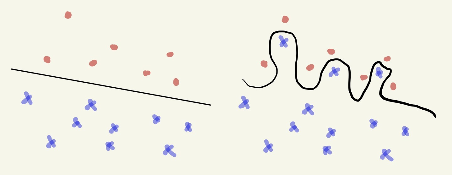
The loss function is not differential!
위 사진에서 왼쪽같은 경우는 Simple classification 모델을 통해 분류하는 것이 가능하다.
하지만 오른쪽은 어떤 선을 긋더라도 두 개의 클래스를 분류할 수 없는 경우가 존재한다.
이러한 케이스에서 Simple classification 을 통해 문제를 해결할 수 없다.
※ Probabilistic View for a Linear Classifier
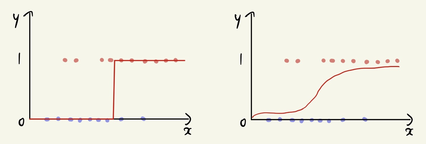
What if we consider the output as \(P(y = 1|x)\) ?
- As \(h(x)\) is close to 1, x is more likely to be 1 (Red).
- As \(h(x)\) is close to 0, x is more likely to be 0 (Blue).
\(h(x) = \begin{cases} 1 (Red) & \text{ if } f(x) \geq 0 \\ 0 (Blue) & \text{ otherwise } \end{cases} \Rightarrow h(x) = \frac{1}{1 + exp(-f(x))}\)
주어진 data가 positive 샘플인 경우, 주어진 확률이 최대화되는 방향으로 w 값을 조정한다.
반면에 주어진 data가 negative 샘플인 경우, 주어진 확률이 최소화되는 방향으로 w 값을 조정한다.
즉, 모든 샘플에 대해 각각의 확률들을 계산하고 각각의 확률들이 positive 인 경우엔 최대화되고
negative 인 경우에는 최소화되는 방향으로 w 를 조정하는 것이 목적이다.
\(h(x) = \frac{1}{1 + exp(-f(x))}\) 함수를 Sigmoid 또는 Logistic function 이라고 부르며,
장점으로는 모든 점에서 미분이 가능하다는 점이다.
\(h(x)\) can be interpreted as the probability of "being red."
- As x goes upward from \(f(x), x\) is more likely to be 1 (Red).
- As x goes downward from \(f(x), x\) is more likely to be 0 (Blue).
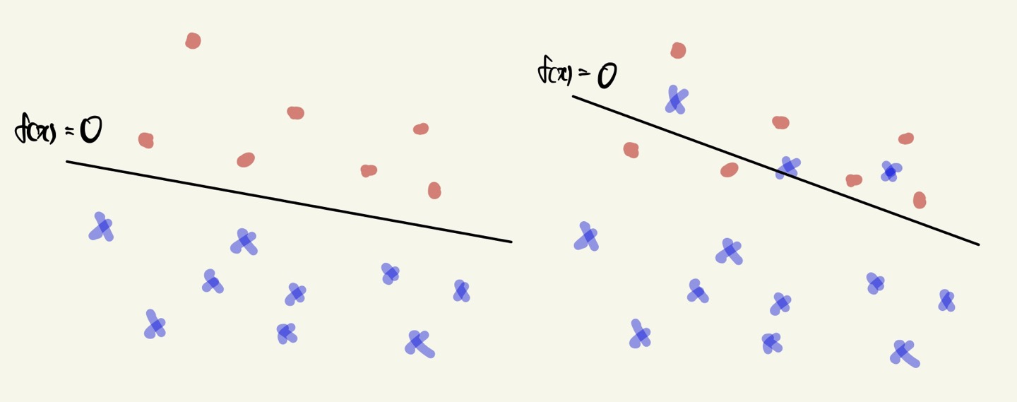
기존의 방식은 선보다 위쪽에 있으면 1, 아래쪽에 있으면 0으로 간주하였다.
다른 방식으로 확률 기반으로서 각각의 점들을 해석한다면 선 위에 점이 존재한다면 그 점의 확률은
\(P(y = 1 | x)\) 에 대한 확률이므로 0.5 로 해석할 수 있다.
그리고 선 위에 점의 확률은 0.6, 0.9 등이 될 수 있고 선 아래에 점의 확률은 0.3, 0.15 등이 될 수 있다.
선과 점 사이의 거리가 멀어질 수록 차이값이 커진다는 점이 있다.
하지만 잘못 분류된 경우에도 동일하게 확률값을 부여할 수 있다.
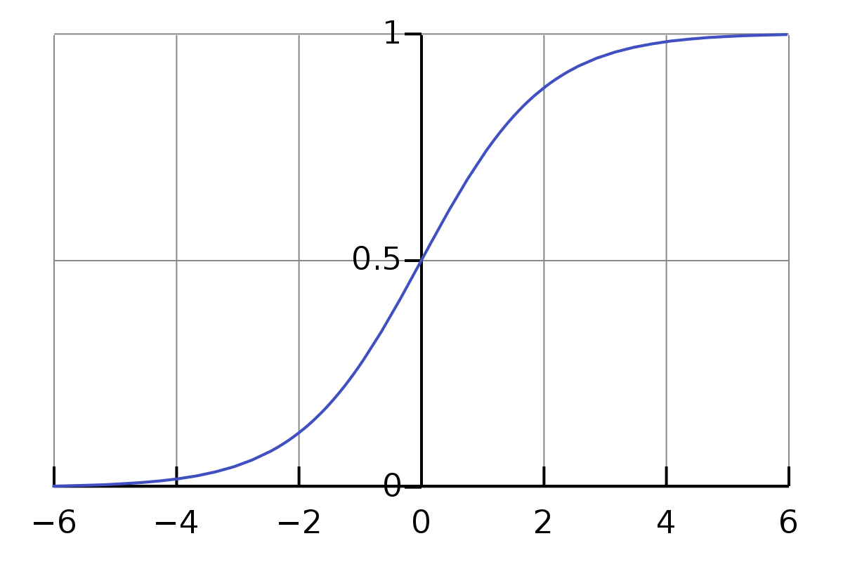
※ What is the Sigmoid Function?
The sigmoid function is a S-curve shape.
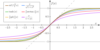
특징으로 다음과 같다.
(1) y 값이 바운드된다. ([-1, 1])
(2) 모든 점에 대해서 미분 가능하다.
(3) 인풋으로 -INF 부터 INF 까지 존재한다.
(4) 모든 미분값에 대해 0보다 크거나 같다.
Logistic function
\(\sigma (x) = \frac{L}{1 + e^{-k(x - x_{0})}} \)
- \(x_{0}\) : the midpoint of the x-value
- L : the curve's maximum value
- k : the steepness of the curve
As the input of the logistic function, \(f(x) = w^{T}x\) is used.
\(h(x) = g(f(x)) = \sigma (f(x)) = \frac{1}{1 + e^{-f(x)}} = \frac{1}{1 + e^{-w^{T}x}}\)
※ Visualizing Geometric Interpretation
A linear decision boundary can be represented as a non-linear logistic function.
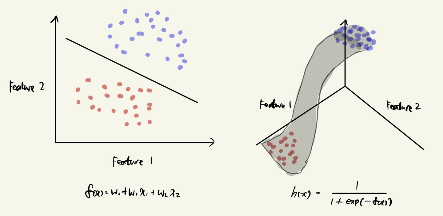
왼쪽은 projection 한 경우로 하나의 직선을 찾는 문제로 logistic regression 을 바라볼 수 있다.
오른쪽은 y 를 추가한 경우로 비선형 형태의 함수에 대해 각각의 점을 projection 하는 것으로 바라볼 수 있다.
Formulating Logistic Regression
※ Formulating Logistic Regression
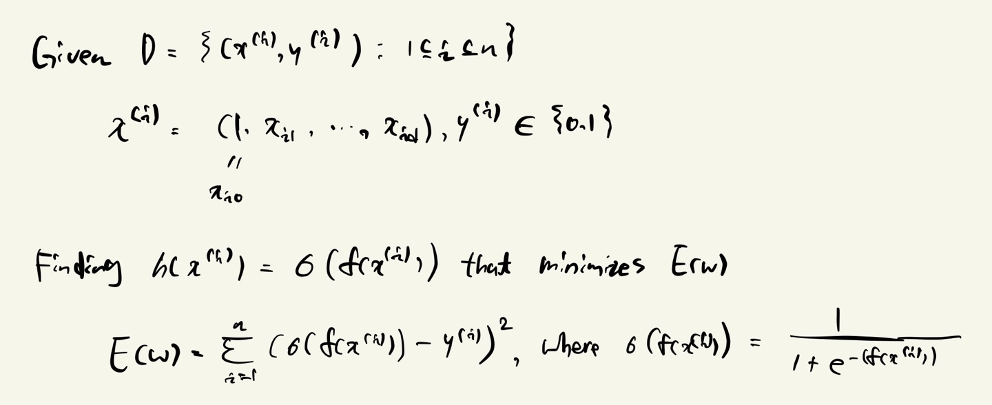
Simply, use the error function used in linear regression.
- \(E(w) = \sum_{i=1}^{n}\left ( \sigma (x^{(i)})-y^{(i)} \right )^{2}\)
This gives the non-convex function for w, which does not guarantee the best minimum.
반드시 global optimal 에 다가갈 수 없다. (non-convex function 이므로)
※ Probabilistic View: Linear Classifier
\(h(x)\) can be interpreted as the probability of "being red."
- As \(x\) goes upward from \(f(x)\), \(x\) is more likely to be 1 (Red).
- As \(x\) goes downward from \(f(x)\), \(x\) is more likely to be 0 (Blue).
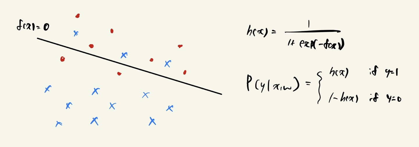
y가 1인 경우 h(x), y가 0인 경우 1-h(x) 으로 볼 수 있다.
각각 확률값을 부여하며, w값에 의해 확률값이 조정되어진다.
예를 들어 검은색 선 0.5 을 기준으로 빨간색 점이 선 위에 존재하면 0.5 초과의 확률값을 보유하고,
선 아래에 존재할 경우 0.5 미만의 확률값을 보유하게 된다.
※ Maximum Likelihood Estimation (MLE)
Estimate the maximum likelihood given independent observations \(x^{(1)}, ..., x^{(n)}\).
\(\zeta (\Theta ) = \prod_{i=1}^{n} f(x^{(i)} | \Theta ) \)
What \(\Theta\) maximizes the likelihood of the observed data?
\(\frac{\partial }{\partial \Theta }\zeta (\Theta ) =0 \)
세타값을 잘 조정하여 최대화할 수 있도록 하는 것이 목표이다.
MLE 모양에 대해 살펴보도록 하자.
※ Formulating the Error Function
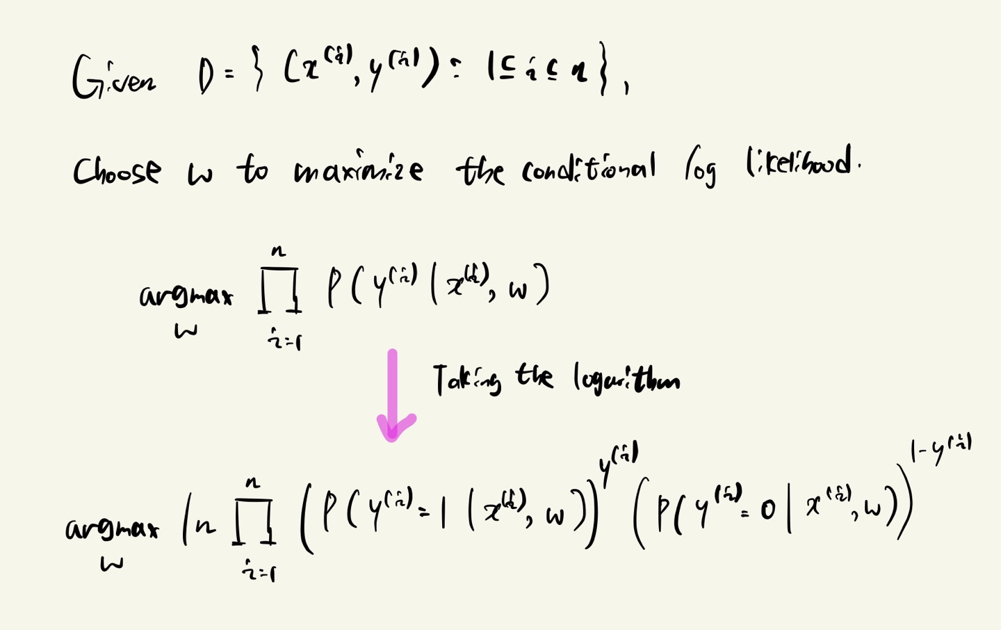
각각 independent 하므로 합이 아닌 곱의 형태로 이루어진다.
이를 로그화하면 위와 같은 식이 나타난다.
결국 로그 안의 곱의 형태는 각 로그의 합의 형태로 풀어서 쓸 수 있어서 계산 편의에 용이하다.
Find a boundary which makes
- Positive samples are likely to be \(P(y = 1 | x, w) \)
- Negative samples are likely to be \(P(y = 0 | x, w) \)
\(P(y = 0 | x, w) \) 는 다르게 표현하자면 \(1 - P(y = 1 | x, w) \) 으로 표현 가능하다.
Find w that maximizes
\( \underset{w}{argmax}\left ( \prod_{x | y = 1}^{}P(y=1|x, w) \right )\left( \prod_{x | y = 0}^{}P(y=0|x, w) \right ) \)
y = 1 에 대한 곱의 형태를 Positive samples,
y = 0 에 대한 곱의 형태를 Negative samples 으로 볼 수 있다.
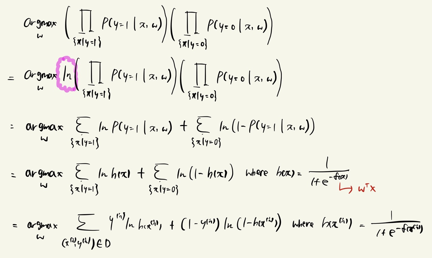
위와 같이 표현한 식이 logistic regression 을 풀 때 사용하는 error function 이 되겠다.
How to solve this?
- A closed form equation
- Gradient descent method
Bad news : There is no closed-form solution to minimize the error function.
\(E(w) = -\sum_{(x^{(i)}, y^{(i)})\in D}^{} y^{(i)}lnh(x^{(i)}) + (1-y^{(i)})ln(1-h(x^{(i)}))\)
위 식은 - 을 붙여서 minimization 을 푸는 방식으로 살짝 변형한 것이다.
그러나 위 식은 closed-form 이 존재하지 않음이 증명되었다.
Good news : The error function is convex!
- Unique maximum : The convex function is easy to optimize.
\(E(w) = -\sum_{(x^{(i)}, y^{(i)})\in D}^{} y^{(i)}lnh(x^{(i)}) + (1-y^{(i)})ln(1-h(x^{(i)}))\)
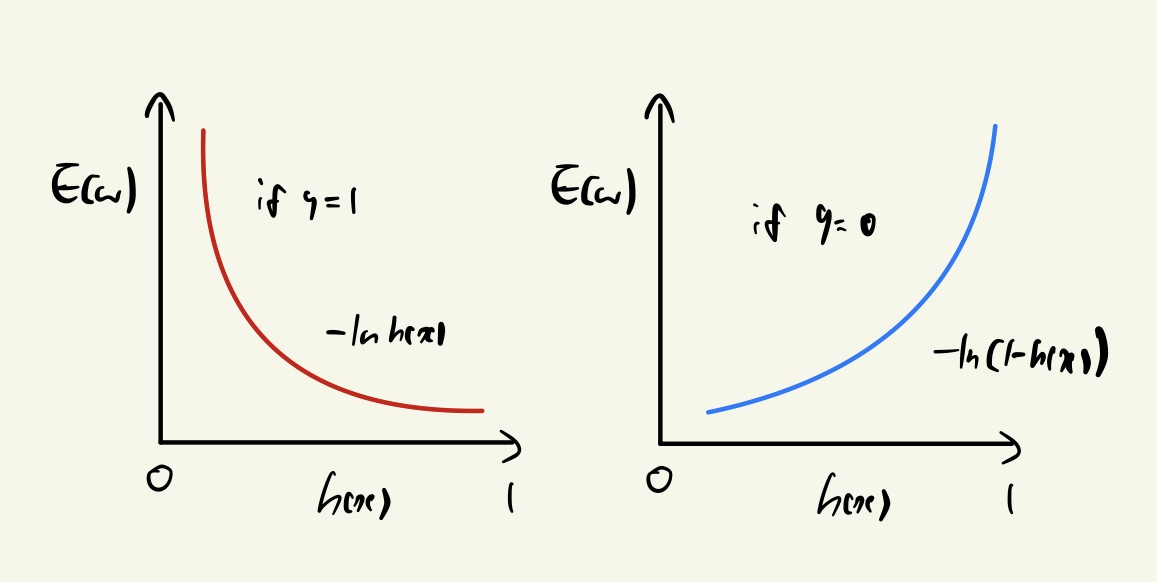
다행히도 로그함수로 표현되기 때문에 convex function 임이 보장된다.
따라서 gradient descent 방법을 이용하여 최적의 해를 찾을 수 있게 된다.
Training Logistic Regression
※ Gradient Descent (GD)
Simple concept: follow the gradient downhill
Process
(1) Pick a start position: \(w^{0} = (w_{0}, ..., w_{d}) \)
(2) Determine the descent direction: \(\Delta w = \bigtriangledown E(w^{t}) \)
(3) Choose a learning rate: \(\eta\)
(4) Update your position: \(w^{t + 1} = w^{t} - \eta \Delta w\)
(5) Repeat from 2) until stopping criterion-is satisfied.
Randomly choose an initial solution \(w^{0}\),
Repeat
Choose a random sample set \( B \subseteq D \)
\( \bigtriangleup w = \sum_{ (x^{(i)}, y^{(i)}) \in B }^{} (h(x^{(i)}) - y^{(i)}) x^{(i)} \)
\( w^{t + 1} = w^{t} - \eta \bigtriangleup w \)
Until stopping condition is satisfied.
※ Computing the Partial Derivative
Using a chain rule.
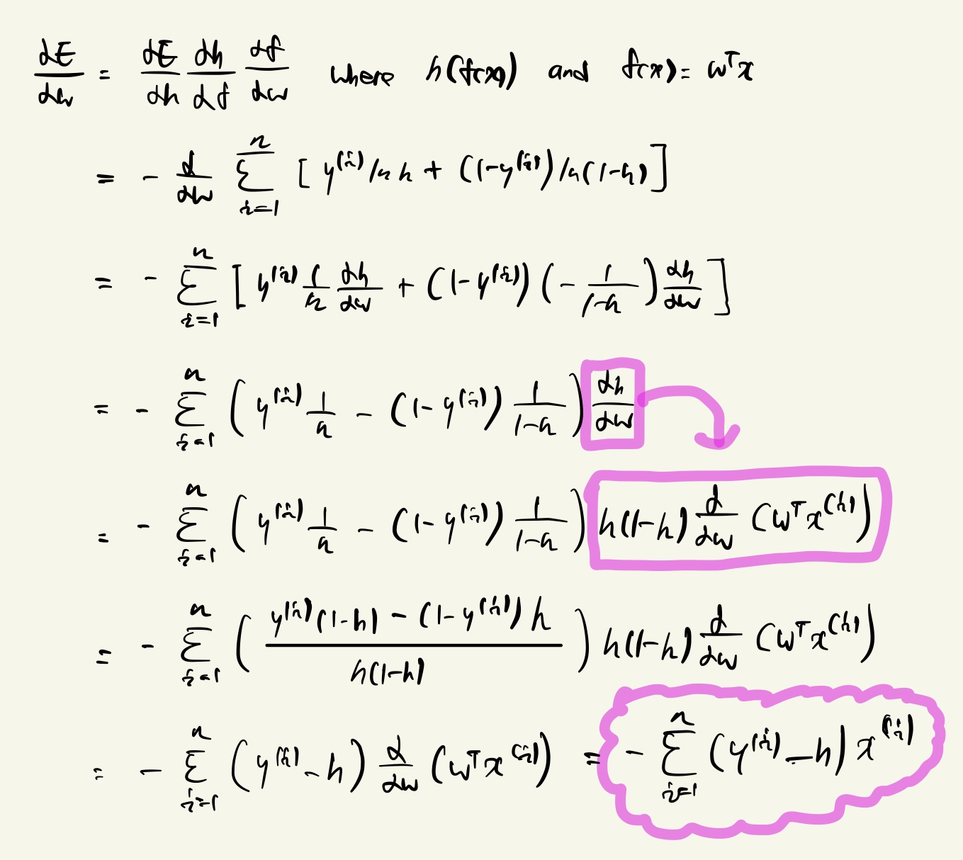
Error function 에 대한 미분결과는 위와 같다.
그러나 \( \frac{\partial h}{\partial w} \) 이 위와 같이 어떻게 유도 되었는지를 살펴보려고 한다.
Denote the sigmoid function as \(\sigma (x) = \frac{1}{1 + e^{-x}} \)
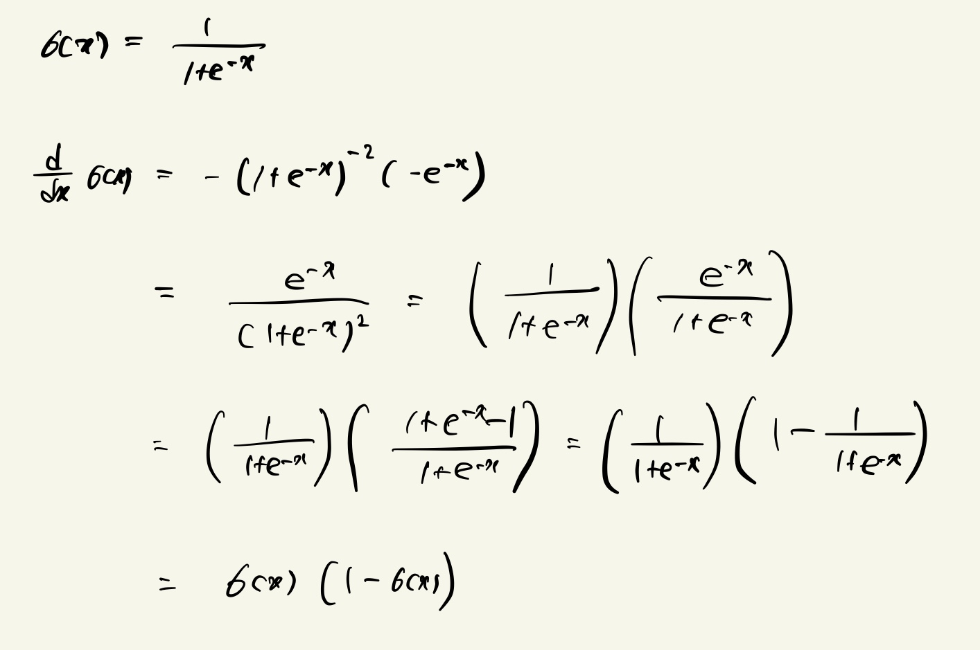
logistic function 을 미분한 결과가 위와 같이 나오므로,
\( \frac{\partial h}{\partial w} \) 의 결과에서 \(h(1 - h)\) 이 어떻게 나왔는지를 알 수 있다.
The error function for logistic regression is
\(E(w) = -\left ( \sum _{(x^{(i)}, y^{(i)}\in D)} y^{(i)}lnh(x^{(i)}) + (1 - y^{(i)})ln(1-h(x^{(i)})) \right )\)
\(h(x) = \sigma (f(x)) = \frac{1}{1 + e^{(-f(x))}} = \frac {1}{1 + e^{-(w_{0}x_{0} + w_{1}x_{1} + ... + w_{d}x_{d})}}\)
The partial derivative of \(E(w)\) is
\(\frac {\partial }{\partial w}E(w) = \sum _{(x^{(i)}, y^{(i)}) \in D} (h(x^{(i)}) - y^{(i)})x^{(i)}\)
이렇게 정리되면, gradient descent 에 적용하면 된다.
'머신러닝' 카테고리의 다른 글
| The Overfitting Problem (0) | 2023.04.03 |
|---|---|
| Multinomial Logistic Regression (0) | 2023.03.29 |
| Parameter Estimation (0) | 2023.03.21 |
| Classification Problem (0) | 2023.03.19 |
| Linear Regression Models (0) | 2023.03.19 |


